Team of four · Data science · MBAN 6110T, Schulich

Ames housing price model

A regression and classification study on 2,930 Ames, Iowa home sales, built with three MMAI teammates as a valuation teaching tool for new real estate professionals. We cleaned the data, engineered eight new features, and benchmarked six regression and four classification models through a single leak-free pipeline to find out which property attributes actually move price, and by how much.

$19,833Ridge regression RMSE
— ~12% of median price
0.913R² — share of price
variance explained
0.938Best classifier F1
— premium vs. standard

The problem

Teaching valuation where it's actually visible

New agents usually learn pricing by watching a mentor work a handful of deals. We built a transparent model trained on real transactions instead.

We chose Ames, Iowa on purpose. In major cities, location dominates pricing so completely that "location, location, location" drowns out every other factor. In a mid-sized college town, the separate contributions of quality, size, age, and neighborhood are visible and measurable, which makes it a better teaching case. We framed the work as two complementary tasks: a regression predicting a home's final sale price, and a classification identifying whether it sells above the market median of $160,000 — a "premium vs. standard" call that mirrors how agents actually triage listings before anyone needs an exact number.

We set three hypotheses before touching a model:

  • H1 — overall quality and above-ground living area will be the strongest price predictors.
  • H2 — sale price will be right-skewed with notable outliers, favoring a log-transformed target for linear models.
  • H3 — neighborhood will explain a substantial share of price variance, reflecting a location premium.

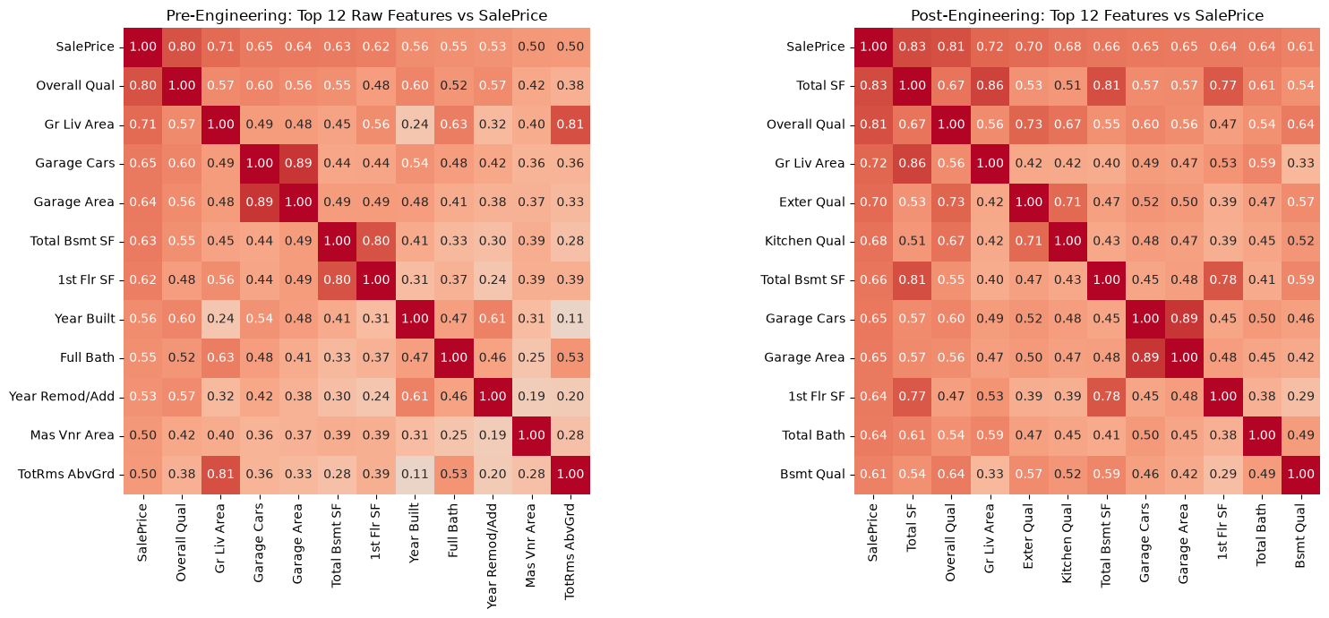
Two correlation heatmaps of the top 12 features against sale price, before and after feature engineering.

Correlation with sale price, before and after feature engineering. The new Total SF feature becomes the single strongest predictor.

Data & cleaning

2,930 sales, 80 features, mostly-structural gaps

Twenty-seven of the 80 columns had missing values, but almost all of it was structural, not random: a blank Pool QC or Garage Area means the feature doesn't exist on that property, not that it went unrecorded. We filled those with an explicit "None" category or 0, rather than imputing a plausible value onto a feature that isn't there.

Lot Frontage was the one genuinely missing variable (~17% of rows), so we imputed it with the neighborhood median rather than the global one. Following the dataset author's own guidance, we also removed five extreme homes over 4,000 sq ft, three of which sold far below what their size and quality implied — non-market sales that would otherwise drag a regression line toward themselves.
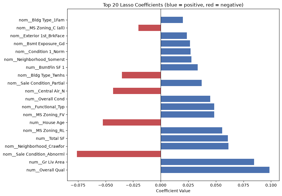

Bar chart of the top 20 Lasso regression coefficients, colored by positive or negative direction.

Top 20 Lasso coefficients. Lasso drove 200 of 276 features to exactly zero, keeping only the ones that add real signal.

Feature engineering

Eight new features, a leak-free pipeline

We combined related raw columns into eight engineered features — Total SF, House Age, Years Since Remod, a weighted Total Bath count, Total Porch SF, and binary flags for pool, garage, and fireplace. Quality columns with a genuine rank order were ordinally encoded; nominal categories like Neighborhood, which have no inherent ranking, were one-hot encoded instead.

Sale price itself was heavily right-skewed (skew = 1.74), so we log-transformed the target and converted predictions back to dollars before reporting error. To avoid leakage, every imputer, scaler and encoder was fit only on the training fold inside a scikit-learn pipeline passed whole into GridSearchCV.


Model results

Ten tuned models, one pipeline

Ridge and logistic regression were our pre-registered picks based on EDA — both finished on top.

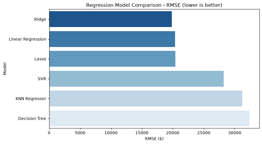
Regression — test RMSE, lower is better

Model RMSE ($) R²
Ridge (α = 10) 19,833 0.913
Linear Regression 20,348 0.899
Lasso 20,395 0.909
SVR (RBF, C = 1) 28,233 0.887
KNN Regressor (k = 7) 31,215 0.836
Decision Tree (depth 10) 32,364 0.789
Horizontal bar chart comparing test RMSE across six regression models, Ridge lowest.

Classification — premium vs. standard

Model Acc. Prec. Recall F1 ROC AUC
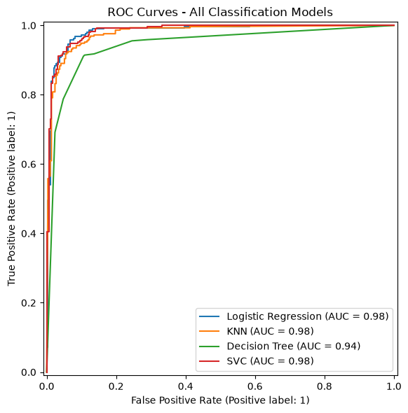
Logistic Reg. (C = 0.1) 0.939 0.938 0.938 0.938 0.983
SVC (RBF) 0.939 0.938 0.938 0.938 0.985
KNN (k = 21) 0.925 0.946 0.901 0.923 0.978
Decision Tree (depth 3) 0.903 0.896 0.911 0.903 0.943
ROC curves for all four classification models, logistic regression and SVC tracking closely near the top-left corner.

Diagnostics

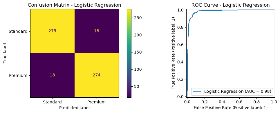
Confusion matrix and ROC curve for logistic regression, showing 275 true negatives, 274 true positives, 18 false positives, 18 false negatives.
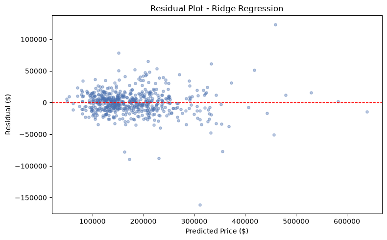
Scatter plot of Ridge regression residuals against predicted price, centered around zero with no clear pattern.

Left: logistic regression's confusion matrix — 18 misclassifications in each direction out of 585 test homes. Right: Ridge's residuals sit centered on zero across the full price range, with no systematic bias at higher prices.

Key finding

What a home is built like matters more than where it is built

Quality-rating columns outranked Neighborhood as price separators in our ANOVA analysis, despite neighborhood having 26 categories to work with against 4–5 for each quality field. That directly challenges the "location, location, location" instinct most new real estate professionals bring to the job — and it's the instructive result the Ames dataset was chosen to surface.

  • H1Supported — Overall Qual (r = 0.80) and the engineered Total SF became the strongest predictors of price.
  • H2Supported — SalePrice was right-skewed at 1.74; the log transform materially improved every linear model.
  • H3Not supported — neighborhood was statistically significant but was outranked by quality ratings as a price separator.

One caveat we're upfront about: the data spans 2006–2010, a window that includes the 2008 financial crisis, so absolute price levels reflect an unusual period. The tool teaches the mechanics of valuation — which features matter and how models weigh them — rather than current market prices; retraining on recent data would be needed before any real deployment.

Team

MBAN 6110T, Schulich

  • Quan Nguyen, Maxwell Levy, Nicholas Scarcelli, Sai Balakrishna Saiprasad. My contribution spanned data cleaning, feature engineering, the regularized regression modeling (Ridge / Lasso), and the results writeup.

References

Sources

  • De Cock, D. (2011). Ames, Iowa: Alternative to the Boston Housing Data as an End of Semester Regression Project. Journal of Statistics Education, 19(3).
  • Pedregosa, F., et al. (2011). Scikit-learn: Machine Learning in Python. Journal of Machine Learning Research, 12, 2825–2830.